Kernelizing Bayesian Linear Regression (Gaussian Process Regression)
Preface
Read Kernel Trick in Machine Learning for context.
Definition
We expand up to a large number of features \(\boldsymbol{\phi}(\mathbf{x})\), and then reformulate so that we only have \(\boldsymbol{\phi}(\mathbf{x})\boldsymbol{\phi}(\mathbf{x'})^{\top}\), ie. the dot product between the two.
Note that \(\mathbf{x'}\) isn't the derivative, it denotes another input point. Saying \(\boldsymbol{\phi}(\mathbf{x})\boldsymbol{\phi}(\mathbf{x'})^{\top}\) is equivalent to saying \(\boldsymbol{\phi}(\mathbf{x}_{i})\boldsymbol{\phi}(\mathbf{x}_{j})^{\top}\), but in a more general sense for any two inputs \(\mathbf{x}\) and \(\mathbf{x'}\).
We also include the prior parameter \(\boldsymbol{\Lambda}_{0}\) into this dot product to get a weighted dot product: \(\boldsymbol{\phi}(\mathbf{x})\boldsymbol{\Lambda}_{0}\boldsymbol{\phi}(\mathbf{x'})^{\top}\).
This weighted dot product corresponds to the kernel function \(\mathbf{k}(\mathbf{x}, \mathbf{x}')\). (This is what is done in Gaussian Process Regression).
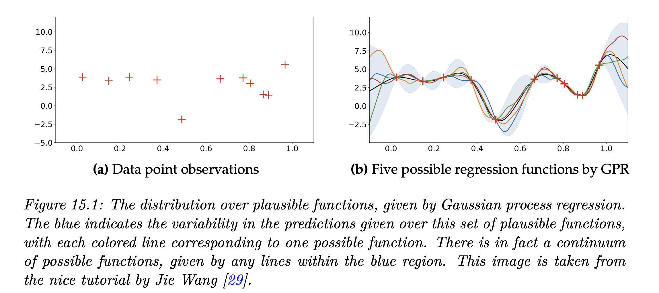 { width="500" }
The choice of \(\boldsymbol{\Lambda}_{0}\) defines the width of the activation region of the kernel. For example, in an RBF kernel, we use \(\Lambda_{0} = \lambda \mathbf{I}\) and have \(\exp\left( -\frac{\lambda}{2}||\mathbf{x} - \mathbf{x}'||_{2}^2 \right)\).
Think of \(\lambda^{-1}\) as the width of the activation:
- Smaller \(\lambda\) corresponds to a wider "activation width": which means that the inputs \(\mathbf{x'}\) that are far from \(\mathbf{x}\) still have non-negligible values in \(\mathbf{k}(\mathbf{x}, \mathbf{x'})\).
-
Bigger \(\lambda\) result to a smaller "activation width", so only values \(\mathbf{x'}\) near \(\mathbf{x}\) have non-negligible activation.
To visualize this "activation width" concept, think of it as a "blurry spotlight" centered at \(\mathbf{x}\), where the width of the spotlight beam is controlled by \(\mathbf{\lambda^{-1}}\). And the brightness at some other point \(\mathbf{x'}\) is given by \(\mathbf{k}(\mathbf{x}, \mathbf{x'})\), which decays with distance from \(\mathbf{x}\).
Now lets see how Gaussian Process's maintain \(p(f(\mathbf{x})| \mathcal{D})\):
- Let the dataset be composed of \(\mathbf{X} \in \mathbb{R}^{n \times d}\) and targets \(\mathbf{y}\in \mathbb{R}^{n}\).
- For any \(\mathbf{x}\), which doesn't need to be in the training set, let \(k(\mathbf{x}, \mathbf{X}) = [k(\mathbf{x_{1}}, \mathbf{x}), \ k(\mathbf{x}_{2},\mathbf{x}), \dots, k(\mathbf{x}_{n}, \mathbf{x})]\) be the vector of kernel (similarity) values between \(\mathbf{x}\) and each training datapoint \(\mathbf{x}_{i}\).
- Let \(\mathbf{K} = k(\mathbf{X}, \mathbf{X}) \in \mathbb{R}^{n\times n}\) be the kernel matrix for our training dataset.
Then we have that:
This formula assumes we have \(\sigma^2\). Recall that \(\sigma^2\) is the variance in \(y\), ie. the inherent noise in \(y\). That is:
In the case of Gaussian Process regression, \(\sigma^2\) is a hyperparameter and needs to be tuned. This means that we get to pick \(\sigma^2\). This may seem weird at first: why are we allowed to choose the inherent noise in \(y\)? Isn't this variance the irreducible error? We actually don't control the noise, but GPR requires \(\sigma^2\), so we're saying: "Let's assume the noise in our data is Gaussian with \(\sigma^{2}\), and we'll estimate the best value of \(\sigma^{2}\) that explains our data."