Eigenvalues and Eigenvectors
Preface
Linear transformations on a vector space can take many different forms: expanding or shrinking a vector by a scalar multiple, rotating a vector, reflecting a vector in a hyperplane, permuting components of a vector, etc...
The effect of most linear transformations are a complex mixture of these, but a special few are much simpler in their actions.
We want to break down linear transformations into their most basic building-block actions so that its overall behaviour can be readily understood.
The key issue is what happens when a given linear transformation is applied repeatedly: do the results settle down into some steady state, do they oscillate, or blow up? This question can be answered by breaking down the transformation into expansions or contractions in specific directions.
Definition
A given direction in a vector space is determined by any nonzero vector pointing in that direction. Thus, given an \(n \times n\) matrix \(\mathbf{A}\) representing a linear transformation on an \(n\)-dimensional vector space, we wish to find a nonzero vector \(\mathbf{x}\) and a scalar \(\lambda\) such that
\(\lambda\) is the eigenvalue, how much the direction vector \(\mathbf{x}\) expands or contracts. \(\mathbf{x}\) is the eigenvector, the direction in which this expansion or contraction occurs.
Thus, eigenvalues and eigenvectors provide a means of understanding the transformation of \(\mathbf{A}\), by breaking it down into a sequence of expansions and contractions of different magnitudes in different directions.
Solving for Eigenvalues
First we note that
This homogenous system of linear equations has a nonzero solution \(\mathbf{x}\) if and only if its matrix is singular.
- Singular because we want it such that matrix \(\mathbf{A-\lambda I}\) annihilates certain vectors \(\mathbf{x}\) to \(\mathbf{o}\).
Thus, the eigenvalues of \(\mathbf{A}\) are the values of \(\lambda\) such that
This gives a polynomial of degree \(n\) (since \(\mathbf{A} \in \mathbb{R}^{n\times n}\)) in \(\lambda\), called the characteristic polynomial of \(\mathbf{A}\), and its roots are the eigenvalues of \(\mathbf{A}\).
Example:
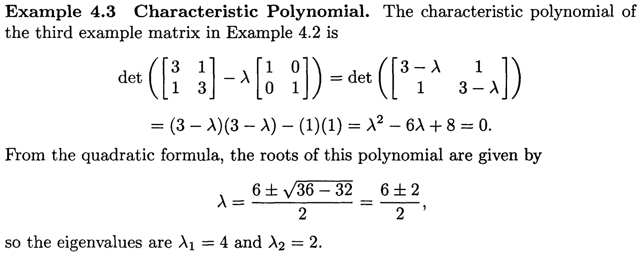 { width="400" .center }
Because the eigenvalues of a matrix are the roots of its characteristic polynomial, which has degree \(n\), we conclude that an \(n \times n\) matrix \(\mathbf{A}\) always has \(n\) eigenvalues, but they may not be real, nor distinct.
Not having distinct eigenvalues simply means that more than one direction can have the same expansion or contraction factor.
However, finding eigenvalues this way is not worth it. There is an iterative process to find eigenvalues called: Power Iteration (computing eigen values and vectors)