Sensitivity and Conditioning of Rectangular Matrices (numerical analysis)¶

Definition¶

The definition of the condition number of a square matrix (Sensitivity and Conditioning of Square Matrices (and amplification factor) 1) doesn't apply to non-square matrices, since their inverse does not exist.

However, we can define a pseudoinverse, denoted as \(\mathbf{A}^{+}\), that behaves like an inverse in many respects.

We are only considering matrices with full column rank (that is, given \(\mathbf{A}\in \mathbb{R}^{m \times n}, \ where \ m>n\), \(\text{rank}(\mathbf{A})=n\)). This means that \(\mathbf{A^{\top}A}\) is non-singular and we define the pseudoinverse as

\[ \mathbf{A}^{+} = (\mathbf{A^{\top}A})^{-1} \mathbf{A}^{\top}. \]

Know that (through some mathematical reasoning), the solution to the least squares problem \(\mathbf{Ax \cong b}\) is given by

\[ \mathbf{x} = \mathbf{A}^{+}\mathbf{b}. \]

We can now define the condition number of an \(m \times n\) matrix with \(\text{rank}(\mathbf{A}) = n\) to be

\[ \text{cond}(\mathbf{A}) = ||\mathbf{A}||_{2} \cdot ||\mathbf{A}^{+}||_{2}. \]

By convention, we set \(\text{cond}(\mathbf{A}) = \infty\) when \(\text{rank}(\mathbf{A}) < n\). And just as the condition number of a square matrix measures the closeness to singularity, the condition number of a rectangular matrix measures the closeness to rank deficiency.

Sensitivity¶

Whereas the conditioning of a square system \(\mathbf{Ax=b}\) depends only on \(\mathbf{A}\), the conditioning of a least squares problem \(\mathbf{Ax \cong b}\) depends on the right-hand-side vector \(\mathbf{b}\) as well as the matrix \(\mathbf{A}\). This means that \(\text{cond}(\mathbf{A})\) alone is not able to characterize the sensitivity of the linear system.

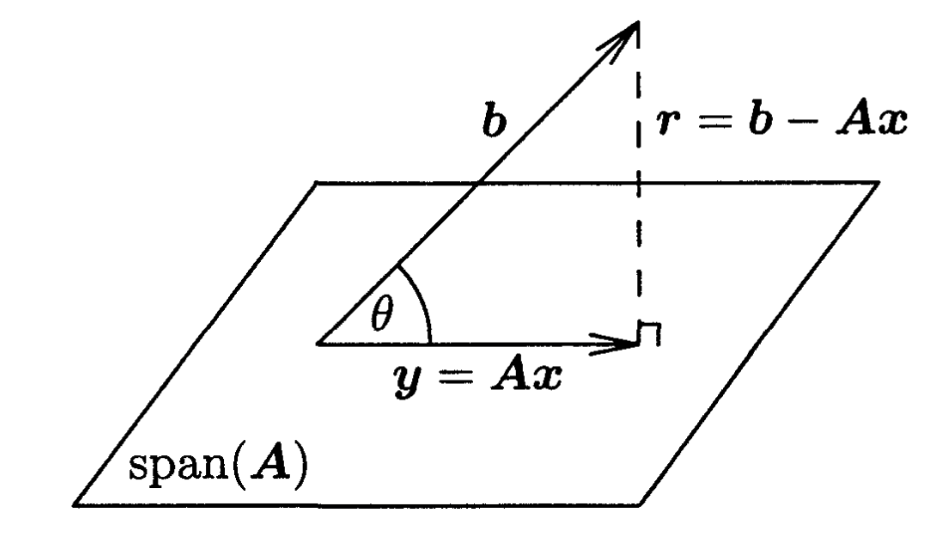
If \(\mathbf{b}\) lies near \(\text{span}(\mathbf{A})\), then a small perturbation in \(\mathbf{b}\) changes \(\mathbf{y = Ax}\) very little. But if \(\mathbf{b}\) is nearly orthogonal to \(\text{span}(\mathbf{A})\), then \(\mathbf{y}\) is relatively small (refer to image). This means a small change in \(\mathbf{b}\) can cause a relatively large change in \(\mathbf{y}\), and hence in the solution \(\mathbf{x}\).

{ width="300" .center }

Thus, for a given \(\mathbf{A}\), we expect the least squares problem with a \(\mathbf{b}\) that results in a large residual (poor fit to data) to be more sensitive than a \(\mathbf{b}\) that results in a small residual (good fit to data). An appropriate measure of the closeness of \(\mathbf{b}\) to \(\text{span}(\mathbf{A})\) is the ratio:

\[ \frac{||\mathbf{Ax}||_{2}}{||\mathbf{b}||_{2}} = \frac{||\mathbf{y}||_{2}}{||\mathbf{b}||_{2}} = \cos(\theta), \]

where \(\theta\) is the angle between \(\mathbf{b}\) and \(\text{span}(\mathbf{A})\).

References¶

Linear Least Squares Problems Overdetermined System (numerical analysis)