Nonlinear Equations
Definition
The most natural way to write a general nonlinear equation would be \(\mathbf{f(x) = y}\), which asks the question, "For what value of \(\mathbf{x}\) does the nonlinear function \(\mathbf{f(x)}\) take on the value of \(\mathbf{y}\)?"
However, it is more conventional to subtract \(\mathbf{y}\) from both sides and incorporate it into \(\mathbf{f}\), so that the equation can be expressed as
where \(\mathbf{f}: \mathbb{R}^{n} \to \mathbb{R}^{m}\), and we seek a vector \(\mathbf{x}\) such that all of the component functions of \(\mathbf{f(x)}\) are zero simultaneously.
If the system is overdetermined, \(m > n\), then usually there is no solution and we look for an approximation in the least squares sense.
If the solution is underdetermined, \(m < n\), then there are infintely many solutions; which is mainly of interest in constrain optimization problems.
Nonlinear equations can have any number of solutions, due to their curved surfaces being able to intersect in many more ways than linear surfaces can. Thus, it is difficult to gauge the number of solutions a particular nonlinear equation has.
Example
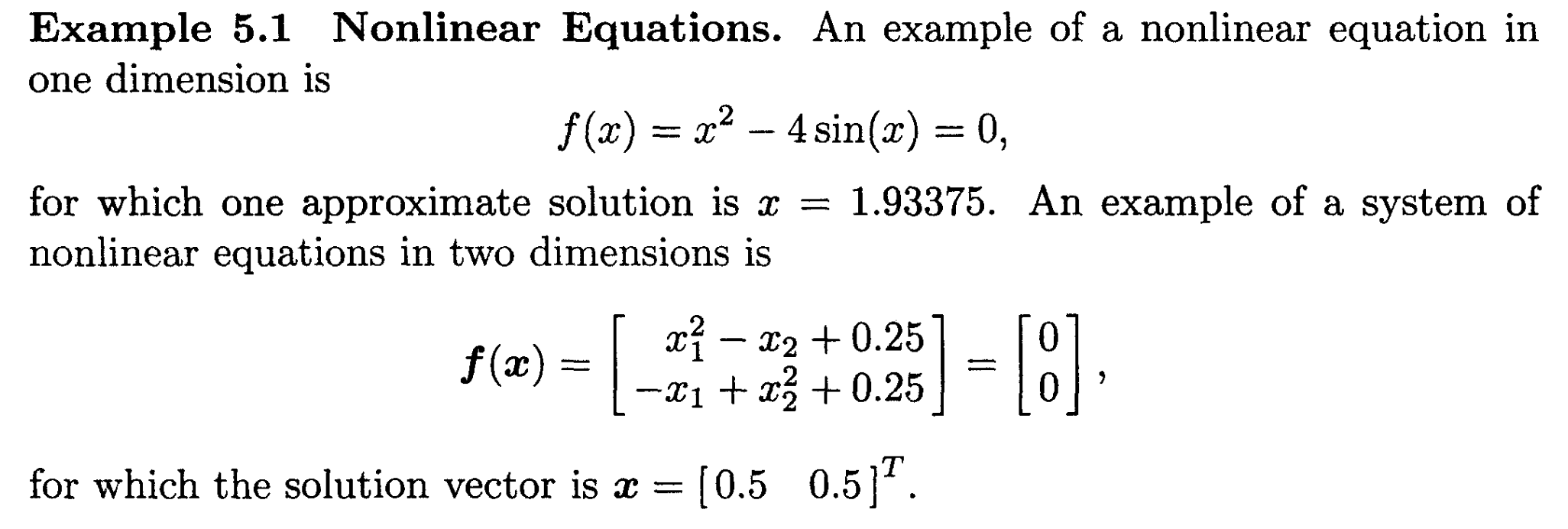
Solutions of Nonlinear Equations in a Local Area
One Dimension
In the one-dimensional case, we can use the Intermediate Value Theorem. As long as we find two endpoints \(a\) and \(b\) that differ in sign, we can guarantee a zero (a solution) to the nonlinear equation.
Such an interval \([a,b]\) is called a bracket. Refining a bracket - ie. making the space between \([a,b]\) smaller - is easy, and there are iterative algorithms to do so. But finding a bracket is a matter of trial and error.
Multiple Dimensions
For n-dimensions we can use the Inverse Function Theorem. If \(\boldsymbol{\mathcal{f}}\) is invertible, then \(\boldsymbol{\mathcal{f}}(\mathbf{x}) = \mathbf{y}\) has a solution for any \(\mathbf{y}\) in that neighbourhood of \(\boldsymbol{\mathcal{f}}(\mathbf{x}^{*})\).
Unfortunately, even if the jacobian \(\mathbf{J}_{f}(\mathbf{x})\) is nonsingular for all \(\mathbf{x} \in \mathbb{R}^{n}\), so that \(\boldsymbol{f}(\mathbf{x})\) is locally invertible anywhere, it still may not be globally invertible in all of \(\mathbb{R}^{n}\) unless some other conditions also hold.
Sensitivity & Conditionin of Nonlinear Equations
Since we want to solve the equation (the root finding problem)
we are essentially finding the inverse problem. That is, for the given value \(\mathbf{y = 0}\), we want to find a value \(\mathbf{x}\) such that \(\boldsymbol{f}(\mathbf{x}) = \mathbf{0}\).
This means that the sensitivity for the root finding problem is opposite to that of evaluating a function. Thus,
- If the function is insensitive to its input, then the root is sensitive.
- If the function is sensitive to its input, then the root is insensitive.
A root being sensitive means the value of the root changes a lot, ie. Let \(x^{*}\) be a root, \(s\).\(t\) \(f(x^{*}) = 0\), then we want to find a \(y=0\) such that
This means any perturbation \(y = 0 + \epsilon\) can cause a drastic change in our computed root.
For a quantitative measure, note that for a root finding problem for \(f\) at \(x^{*}\), the absolute condition number is \(1 / |f'(x^{*})|\). This means that when we have found a point \(\hat{x}\) such that \(|f(\hat{x})| \leq \epsilon\), the error
Thus, when the slope of \(f\) is near zero, the root is sensitive and vice versa.
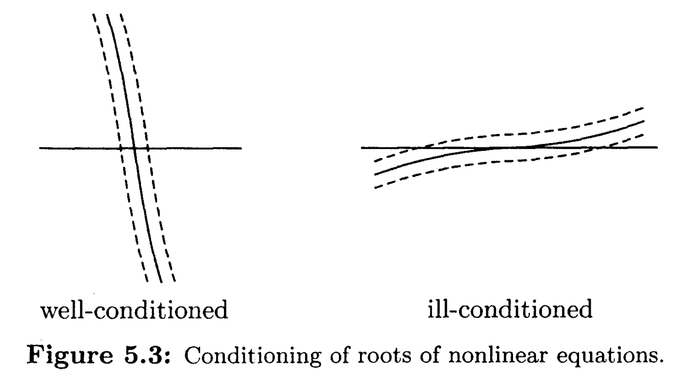 { width="300" .center }
The corresponding absolute condition numbers for function evaluation and root-finding problems are \(||\mathbf{J}_{f}(\mathbf{x}^{*})||\) and \(||\mathbf{J}_{f}^{-1}(\mathbf{x}^{*})||\) respectively.