Bayesian Linear Regression¶

Preface¶

Bayesian Linear Regression involved maintaining the posterior distribution while assuming that the prior \(p(\mathbf{w})\) is Gaussian, and \(p(y|\mathbf{x})\) is a Gaussian with mean \(\mathbf{w^{\top}x}\) and unknown variance \(\sigma_{y}^2\).

The posterior is maintained over \((\mathbf{w}, \sigma_{y})\), and corresponds to a normal-inverse Gamma distribution. This means we are maintaining the distribution \(p(\mathbf{w}, \sigma_{y} | \mathcal{D})\)

Important Note: In the context of Bayesian inference, we denote parameters with subscript 0 as prior parameters. And the subscript \(n\) refers to the parameters after observing \(n\) data points (they are updated values that incorporate evidence from the data).

Definition¶

For Bayesian estimation, we need to maintain the entire posterior, not just the mode.

Computing the posterior is often complicated, unless we have conjugate priors. For Bayesian Linear Regression, where \(p(y | x) = \mathcal{N}(\mu = xw, \sigma_{y}^{2})\), the conjugate prior is the prior used for \(l 2\)-regularization: \(p(w) = \mathcal{N}\left( 0, \frac{\sigma_{y}^{2}}{\lambda} \right)\).

Given this \(p(w)\), where \(\mu_{0} = 0\) and \(\sigma_{0}^2 = \frac{\sigma_{y}^2}{\lambda}\), we derive:

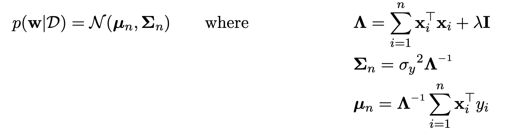
\[ \begin{align} p(w| \mathcal{D}) = \mathcal{N}(\mu_{n}, \sigma_{n}^2) \ \ \text{ where } \ \ \sigma_{n}^2 &= \frac{\sigma_{y}^2}{\sum_{i=1}^n x_{i}^2 + \lambda} \\ \mu_{n} &= \frac{\sum_{i=1}^n x_{i}y_{i} + \lambda \mu_{0}}{\sum_{i=1}^n x_{i}^{2} + \lambda} = \frac{\sum_{i=1}^{n} x_{i} y_{i}}{\sum_{i=1}^{n}x_{i}^2 + \lambda} = \frac{\sigma_{n}^2}{\sigma_{y}^{2}}\sum_{i=1}^n x_{i}y_{i} \end{align} \]

The MAP solution corresponds to the mode of this distribution: \(\mu_{n}\). Additionally, we can obtain a credible interval for which weights are plausible for the given data, given by the variance \(\sigma_{n}^2\). Notice as \(n\) gets larger, the variance \(\sigma_{n}^2\) shrinks We can also get the same derivation for \(p(\mathbf{w}|\mathcal{D})\) in the multivariate case: { width="400" }

Incorporating the Normal-Inverse Gamma¶

For linear regression though, we usually don't know \(\sigma_{y}^{2}\), however we can estimate this variance using the Normal-Inverse Gamma (NIG) distribution, which is the conjugate prior on the weights \(w \in \mathbb{R}\) and also on the variance \(\sigma_{y}^{2}\).

The Normal-Inverse Gamma distribution has four parameters: \(\mu_{n}, \lambda_{n}, a_{n},b _n\). For prior parameters: \(\mu_{0} \in \mathbb{R}\) and \(\lambda_{0}, a_{0}, b_{0} > 0\), then we obtain the posterior:

\[ \begin{align} p(w, \sigma_{y}^2 | \mathcal{D}) = \text{NIG}(\mu_{n}, \lambda_{n}, a_{n}, b_{n}) \ \text{ where } \ \lambda_{n} &= \sum_{i=1}^n x_{i}^2 + \lambda_{0} \\ \mu_{n}&= \frac{\sum_{i=1}^n x_{i}y_{i} + \lambda_{0}\mu_{0}}{\lambda_{n}} \\ a_{n} &= a_{0} + \frac{1}{2} n \\ b_{n} &= b_{0} + \frac{1}{2}\left( \sum_{i=1}^n y_{i}^{2} + \lambda_{0}\mu_{0}^2 - \lambda_{n}\mu_{n}^2\right) \end{align} \]

Notice that \(p(w, \sigma_{y}^{2}) = p(w|\sigma_{y}^{2})\cdot p(\sigma_{y}^2)\). A key property of an NIG distribution \(p(w, \sigma_{y}^2)\) with parameters \(\mu, \lambda, a, b\) is that: \(p(w | \sigma_{y}^{2})\) is a Gaussian \(\mathcal{N}(\mu, \ \sigma_{y}^2 / \lambda)\) and, \(p(\sigma_{y}^{2})\) is an inverse gamma distribution with parameters \(a, b\).

The mode of the NIG distribution is \(\mathbb{E}[(w, \sigma_{y}^2)] = \left( \mu_{n}, \frac{b_{n}}{a_{n}- 1} \right)\). Thus we have an estimate for the variance \(\sigma_{y}^{2} \approx \frac{b_{n}}{a_{n}-1}\), and the solution for \(w\) is the same as for MAP.

We can use this distribution to reason about a plausible set of values over the weights \(w\), called the credible interval. The variance of the weights, more precisely, corresponds to \(\frac{b_{n}}{(a_{n} - 1) \lambda_{n}}\) for \(a_{n} > 1\). If this term is large, the variance is large, and so the set of plausible weights is large.

We can be more precise by computing \(p( w \in [a,b] \ | \ \mathcal{D}) = 0.95\) to get a 95% credible interval for \(w\).

. . .

The above update extends to the multivariate case as well, where we need now a prior on the weight vector \(\mathbf{w}\in \mathbb{R}^d\) and the variance \(\sigma_{y}^{2}\), where the variance is still a scalar, since it is the variance that corresponds to the scaler \(y\) given \(\mathbf{x}\).

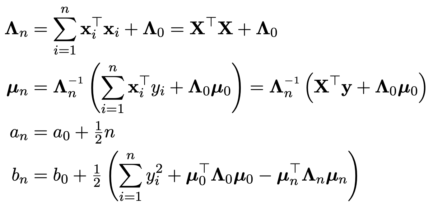
The conjugate prior is still a Normal Inverse Gamma distribution, but now the parameters are: \(\boldsymbol{\mu}_{n} \in \mathbb{R}^{d}, \ \boldsymbol{\Lambda}_{n} \in \mathbb{R}^{d \times d}, a_{n}, b_{n}\).

And the prior parameters are: \(\boldsymbol{\mu}_{0} \in \mathbb{R}^{d}, \ \boldsymbol{\Lambda}_{0} \succeq 0, a_{n},b_{n}>0\). (ie. \(\boldsymbol{\mu}_{0} = 0, \ \boldsymbol{\Lambda}_{0} =\mathbf{I}, \ a_{n} = 3, \ b_{n}= 10\)).

Then we get posterior \(p(\mathbf{w}, \sigma_{y}^2 | \mathcal{D}) = \text{NIG}(\boldsymbol{\mu}_{n}, \boldsymbol{\Lambda}_{n}, a_{n}, b_{n})\) where: { width="400" }

Thus, the covariance of the weights, under the NIG, corresponds to \(\frac{b_{n}}{a_{n}- 1} \boldsymbol{\Lambda}_{n}^{-1}\) for \(a_{n} > 1\).

However, we want more than this. We want to find a credible interval over our predictions \(f(\mathbf{x})\). Namely, given \(p(\mathbf{w}| \mathcal{D})\), we would like to reason about \(p(f(\mathbf{x})|\mathcal{D})\) where \(f(\mathbf{x}) = \mathbf{xw}\) for any \(\mathbf{x}\). See: Uncertainty in Predictions via Bayesian Inference

References¶

Normal-Inverse Gamma Distribution Conjugate Prior Maximum A Posteriori (MAP) Normal-Inverse Gamma Distribution